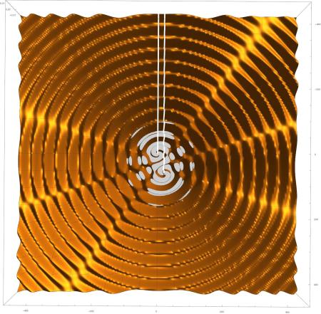
Here are actual computed results of how the interference pattern moves for a dual interference source. In my previous post, I described how a moving interference pattern will alter the location displacement of the interference sources, which leads to the conclusion that quantum interference should enable stable solitons. There, I showed a schematic representation of what should happen. Here is visual computed proof that what I described actually happens: The first picture shows no orthogonal displacement of the interference sources, so the interference paths are symmetric about the interference source X axis. However, the following pictures demonstrate more and more successive orthogonal Y displacement, causing the interference peak paths to rotate in such a way as to displace the nearby interference source. This assumes that the interference source will follow the rotating interference path–we know this is true due to experimental verification via the two-slit experiment as one example. As a result, you should see that moving one interference source should cause the adjacent interference source to move in the opposite direction, causing the two sources to orbit like a binary star (see the previous post for details).
Notice the white line, this is the X axis reference direction to help assess the interference path rotation as y-axis displacement is added to one of the interference sources. These examples show just one possible interference system–it shouldn’t be unreasonable that I conclude that all planar non-degenerate interference cases should behave the same way. Things get really interesting when one of the sources is rotated into the Z axis, and when a third source is placed on the Z axis, and when the wavelength of one of the sources is doubled or multiplied by other factors such as 1/3 or 2/3. More to come…
Agemoz
Edit: My initial analysis (see previous post) showed that the two interfering sources would cause a rotating interference pattern if one were to move past the other in the direction orthogonal to the axis that both sources lie on. I could show that there would be an induced motion to the second source if the first source were moved orthogonally, but did not know what would keep the second source from moving centripetally (moving away from the center). Closer examination (see zoomed in picture) shows that there is a potential well in both the X and Y direction–the interference pattern itself is what constrains the radius of the orbiting path. I do not need to invoke something like the speed of light to keep the orbital path confined to its radius.


Edit: My initial analysis (see previous post) showed that the two interfering sources would cause a rotating interference pattern of rays if one were to move past the other in the direction orthogonal to the axis that both sources lie on. I could show that there would be an induced motion to the second source if the first source were moved orthogonally, but did not know what would keep the second source from moving centripetally (moving away from the center). I tried to bring in something, the speed of light, to confine the radius of the interference particle orbit, but soon felt like this was a flaw in my scheme for describing a soliton via interference (this is the same reason that various DeBroglie/Compton schemes using an EM field fail). However, closer examination (see zoomed in picture) shows that the interference pattern is a potential well in both the X and Y direction–the interference pattern itself is what constrains the radius of the orbiting path. The rays in the previous images are actually interference zeroes, not peaks–the particles will follow a path defined by the peaks. I do not need to invoke a contrivance like the speed of light to keep the orbital path confined to its radius.

Agemoz
Tags: physics, quantum, quantum theory, simulation

Leave a comment