Agemoz's Physics Blog

Charged point particles are very interesting because there’s only a few ways to produce stable (static) configurations of them. You cannot create a 2 particle solution or 6 or more particle solutions. Only three solutions exist: an in-line 3 particle solution, a 4 particle solution, and two 5 particle solutions (see the last few previous posts).

UPDATE: I have found that these charge stable particle solutions fall into a single class of solutions with one or two center particles, where the remaining particles have opposite charge and are equally spaced on a sphere about the center particle(s). If there are two center particles, they have to lie equally spaced on a line normal to the plane of a circle on the sphere (therefore, the three particle solution cannot have two center particles since three particles define a plane). I’m continuing to see if there are any other stable solutions, but after quite a bit of thinking, I see no more. The set of stably charged solutions is really small–there is only this class of solutions and no others–and it does appear to have a curious, possibly interesting, mapping to quark combinations as mentioned in the rest of this post.

Continuation of the original post:

This gets really interesting when applied to electrons and quarks. If you do a little “quark algebra” like this (I’m ignoring the relatively tiny neutrino component):

proton = u + u + d

neutron = u + d + d, which decomposes to a proton, e-, and neutrino -> u + u + d+ e- + O(0)

this leads to

d = u + e-

which then gives

proton = u + u + u + e-

neutron = u + u + u + e- + e-

These match two of the available stable charged point particle configurations, so I got very interested in studying this construction–seems like there might be a path to some kind of truth here. However, computing the traditional inter-particle forces q₁q₂/r^2 gives the required charge for the up quark that is not 2/3, but sqrt(3) electron charge.

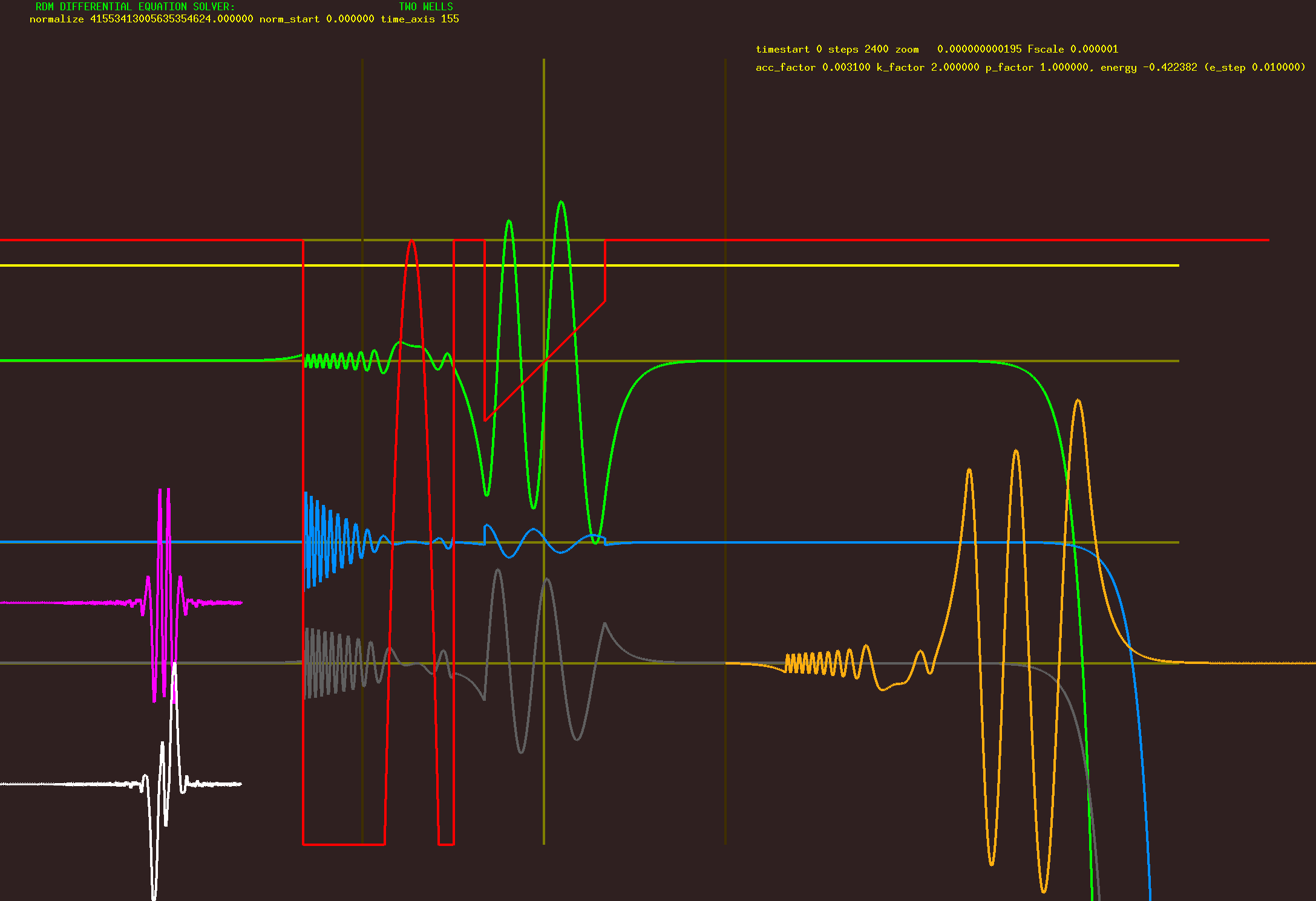
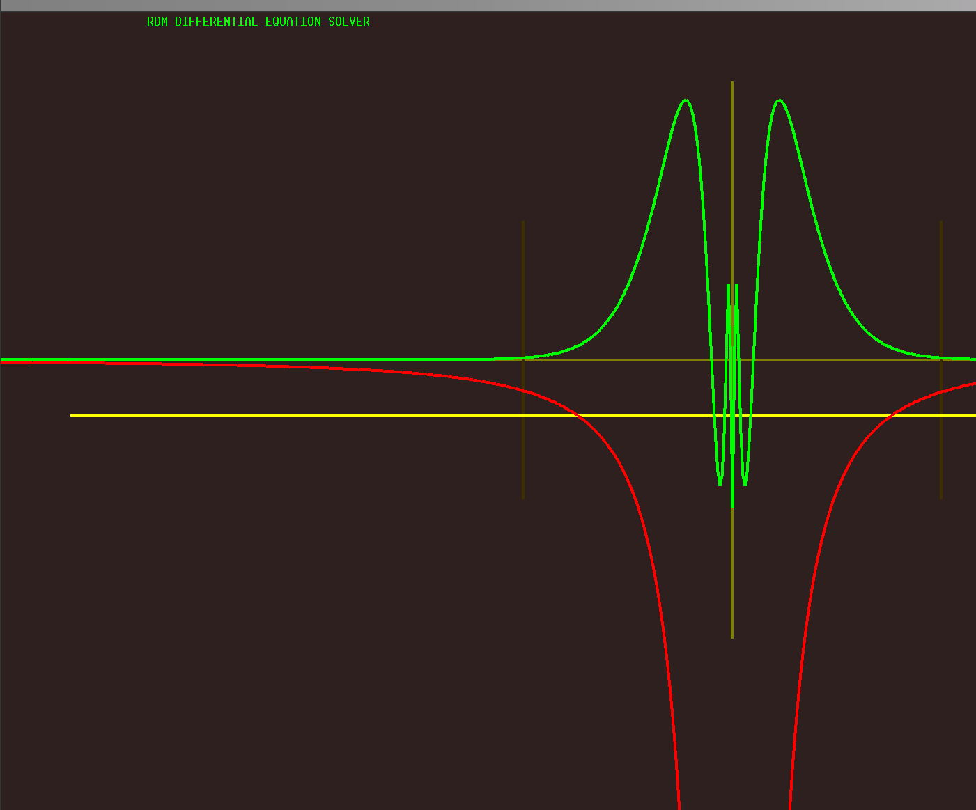
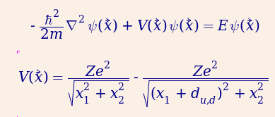
I studied this for a while to see if my Schroedinger wave solver would give some insight, but it didn’t. It did show that one solution is to add a momentum term to Psi for the up quark (implying an orbital), but this did not get anything close to the expected up quark charge.

This problem (getting the correct value for the forces involved) is analogous to the quantum field issues encountered in the electron-photon interaction, and thus is likely to be a hard problem to solve. For example, I am assuming a shielded electron charge, ignoring creation-annihilator effects, ignoring vacuum polarization, ignoring well-researched strong force implications, etc, etc.

Nevertheless, I continued my thought process–I looked in detail at the development of the electron-photon interaction in quantum field theory. It establishes that charged attraction/repulsion is mediated by quantized photons, either virtual or real. On the macroscopic scale we model attraction with a central force (1/r^2) electrostatic field. At the quantum scale, I think there is evidence that something different happens.

I see a very important key with this discovery: any linear force granular particle interaction will always obey the central force property for far-field interactions simply because there is a 1/r^2 diminishing number of particles per square area as you move away from the source emitter. The particle current density in expanding spherical shell surfaces drops as 1/r^2.

This leads to a really important corollary: Individual quantized point particles cannot interact with a central force behavior but must interact linearly with r, otherwise the overall granular central force behavior would produce a composite function that is no longer central force.

This is why I hold the belief that quantum field renormalization is an unnecessary correction for the infinities resulting from central force (1/r^2) functions in quantum field equations as distances approach zero. Renormalization (for example, setting an r threshold or subtraction of infinities to make solutions workable) should not be necessary if we understand that electrostatic forces have a far-field central force behavior (1/r^2 dependence), but in the near-field quantized case must have a linear interaction behavior.

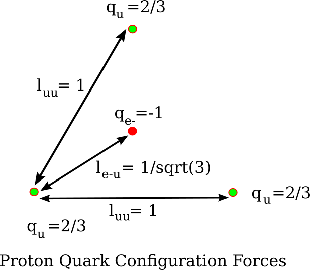
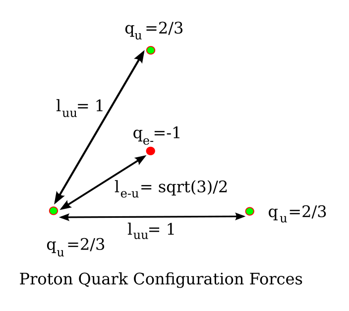
This near-field linear behavior also substantiates my view that the electrostatic central force equation q₁q₂/r^2 is not the right formula for the stable 4 point particle configuration, they must interact as q₁q₂/r. With this correction, we now get closer to the required 2/3 charge for the up quarks.

F_e–_u = 2/3 * 1 * sqrt(3) = 2 / sqrt(3).

F_u–_u = 2/3 * 2/3 * 1 * 2 * sqrt(3) / 2 = 4/3 / sqrt(3))

Now the classical intra-proton quark forces, which must sum to zero if the up quark charge is 2/3, is off by an extra factor of 2/3. I have a number of approaches underway to address this.

One hint comes from unit analysis of the coulomb unit of charge.

Coulomb(SI units) = m/s sqrt(m) sqrt(kg)

There is no physical meaning to a square root of distance (or mass, for that matter) which says to me that charge only has meaning in context with another charge. I did some work a couple of years ago that suggests that near field charges emit and absorb exchange photons that results in a linear force due to point-particle wave interference: see this post

https://wordpress.com/post/agemozphysics.com/1295

I’m going to investigate using this approach on the 4 point-particle proton and see if I get insight as to how charge would work and if I get a correct up quark value in this near-field context.

Agemoz

PS: It is very interesting to me to think about gravity in context with the above-mentioned granular-particle rule and the corresponding central force corollary I discuss. Gravity is, of course, another central-force interaction–but to the best of our knowledge and observations, unlike quantum particles, there is no evidence of linear gravitational behavior at any scale, massive or tiny. I think this may be evidence that gravity is not quantized.

I have found that static point particle charge configurations are rare, and happen to match a geometric construction of quarks in a proton and a neutron. Static charge configurations result from combinations of positive and negative charges that are arranged in stable configurations. There are surprisingly few of these. It is easy to show that in 3 dimensional space (R3) there are no possible two particle solutions, and also that there are no solutions with 6 or more particles. There is a single in-line 3 particle solution, one four particle solution, and two five particle solutions.

What got me especially interested in this line of thought was that a little bit of quark algebra shows that protons and neutrons exactly match the four-particle version and one of the five-particle solutions (see the previous post here for details). I then computed the required charges to form a static configuration for these cases, and thought I came up with the 2/3 charge (relative to the electron -1 charge), but after a lot of rechecking I found some mistakes and realized the required charge value is close, but but does not match. See the updated configuration figure below with a corrected l_e-u. I’m no fan of numerology in physics, so that seemed to blow this exciting idea out of the water–everything has to work right for this concept to be true.

If you look at the figure, you can see the four particle solution, which is a center e- surrounded by three up quarks in an equilateral triangle. The charge forces don’t balance unless the charge is larger than the electron charge, not 2/3. Setting the charge of the up quark to +2/3 results in a force from the electron to the quark of 2 versus a force from the up quark to the other two up quarks equal to 4/(3 sqrt(3)). Numerically the magnitudes are 2.0 versus 0.77, but these have to be exactly equal to produce our geometrically static stable configuration of point particles.

update: arrgh! fixed le-u again, had it right the first time…

I realized that I was applying a classical force model to a quantum wave function system, so I did some simulation work using my Schroedinger wave solver to see if all this would come together to produce the expected charge for this quark construction of the proton and the neutron. This work immediately showed that my static configuration cannot produce a solution unless a momentum term is added. Unfortunately, this complicates things because now we can’t just work with normalized charges–we can assume that the three up quarks orbit the center electron, but now the units involve a momentum term that has no charge factor, so the computation gets more detailed. The momentum term has the usual Schroedinger equation Planck’s constant squared over 2*mass factor, which has to be normalized to the actual charge factor–and now the solution is dependent on radius, the distance between particles in our 4 particle triangle configuration.

The problem has become somewhat more complicated and will require more study which is now underway.

Agemoz

Update: oops. The charge doesn’t come out to exactly 2/3 for the vertex particles. The geometry of charged point particles is very constraining, but the four-particle case leads to a charge that is not exact. Oh, that was a disappointment! I’m rechecking, but looks like this is less useful than I thought.

Update #2: Actually, this result is not surprising–I made the common amateur mistake of applying a classical equation to a quantum (wavefunction) problem. Duh. I’ll be attempting to put the force equation into the Schroedinger wave solver and see what it shows. I don’t want to abandon this work since the matchup of the valid point-particle geometries to real-life quark combinations is still very interesting. The number mismatch is definitely due to using a bad computational methodology, so I don’t want to give up on this.

While it doesn’t really affect anything, I did discover another stable 5 particle solution, a tetrahedron of four particles surrounding a center particle of opposite charge.

(original post) The last month investigation into the R3 + I twist vector field has led to some very interesting insights, such as how particle quantization would work, and why there are 4 elementary point-particle variations, one for each of the spin-up and spin-down electrons and positrons. Quantized photons have their own in-line twist model, where R2 out of the R3 + I provides a frame-independent polarization. Then I made the wonderful discovery that we don’t have to make up a new I rotation dimension for this whole approach–we already have it in the time dimension of spacetime.

So, with this new infrastructure I went back to the Schroedinger Equation problem of protons and neutrons. Previously, I used charged elementary particles (up and down quarks) to attempt to find a time-independent solution. As I reported about a month ago, there are none. But, using my new R3 + I (spacetime) study, I was able to work out a different type of solution that looks very promising.

I did something different this time. Rather than starting with the u,u,d quark configuration of protons, I also looked at free neutrons, which will decay into a proton, an electron, and a neutrino. The neutrino is a very small part of the total proton energy, so if we ignore it (this is one reason why mathematicians dislike physicists 🙂 then we get a different way of constructing the proton. This is just charge geometry. I am pretending the strong force is not at play here, which should be OK if the proton is a lone free particle.

If a neutron is a d,d,u configuration, but decays into a proton plus an electron plus a neutrino, then we could say that

proton = u + u + d + e- + O(0) = neutron = u + d + d

this leads to

d = u + e-

which then gives

proton = u + u + u + e-

Now, there are two statically stable multi-particle configurations, one with four particles and one with five. You can also get one case with three particles in a line, which I investigated a few months ago–but the Schroedinger Equation solver showed no solutions, so I had to rule out that case. Let’s look at the four particle solution:

This is statically stable only if the force between two vertex particles of the triangle is equal to the force from a vertex to the center particle of opposite charge. Let us arbitrarily set the distance between vertices of our equilateral triangle to 1(the ratio of the forces is independent of r, so it doesn’t matter what we set it to). The force between charged particles is proportionate to q1 * q2 / (r * r), so if we put our u particles at the vertices and the e- at the center, the force between the vertex particles is

force(u to u) = 2/3 * 2/3 / (r(u to u) * r(u to u)) = 4 / 9

Now, the force from a vertex to the center particle e- uses an r that is sqrt(3) / 2, so we get

force(u to e-) = 2/3 * (-1) / ((sqrt(3) / 2) * (sqrt(3) / 2)) = 2/3 * 4 / 3 = 8 / 9

Now, don’t forget that each vertex has two other vertices to provide a force component, so lo and behold,

force(u) = -force(u to e-) = 8/9

and thus now we have a stable configuration, the only one possible. You can put whatever you want for r, as long as the vertex charge is -2/3 of the center charge, you will always have a stable solution. Mass doesn’t matter–it affects acceleration, not force, so since this is a static configuration, mass has no effect on the result. This geometry shows why up quarks have to be 2/3 the charge of electrons!

If you look at the neutron using this same analysis, you will get a u + u + u + e- + e-. It turns out there is only one stable 5 particle solution, can you find it? It’s a fun exercise!

Agemoz

Over the years, I have painstakingly worked out how adding a background state directional dimension to R3 enables integer rotations in the field that are quantized. This quantization enables things like quantum photons that observe E=hv and other quantized particles–and recently, I discovered that in R3 + I, point particles have four spin permutations, thus forming a model for the electron variations (spin-up and spin-down electrons and their antiparticles).

In all of this work, I didn’t really consider time as important in developing the rotation state quantization from the R3 + I field. It wasn’t really relevant to the question of point particles or particle quantization. But in the back of my mind, I kept thinking there is something awfully familiar about the properties of the R3 + I field. You probably all saw it before I did, but it suddenly hit me that spacetime has the same (x₀,x₁,x₂,t) vector arrangement as my R3 + I vector rotation field. And, the t component in spacetime, while considered a dimension, is constrained differently than the spatial dimensions–as observers, we are unable to move backwards or forwards in time like we can in space. The dimensional aspect of time shows up in relativistic frame-of-reference situations, where, for example, different observers see different event simultaneity times.

Ignoring the field warping caused by general relativity, spacetime is covered by Minkowski four dimensional geometry with Euclidean axes described by the (x₀,x₁,x₂,t) vector. The rather astonishing discovery I made was that allowing Minkowski field rotations to default to the t dimension direction, quantized twists can form and point particles can exist in the four electron variation forms.

We don’t have to make up a new +I dimension–spacetime itself can form quantized particles and four electron variations!

Agemoz

Electrons come in four variations: spin-up e-, spin-down e-, and their antiparticles, spin-up p+ and spin-down p+. They all are, to the best of our knowledge, point particles and have precisely the same mass and charge magnitude. Throughout the history of physics, DeBroglie and many others tried to create dipoles and other (non-point) configurations to explain these variations but all fail to match experimental observation.

Point particles are a difficult model to work with geometrically in 3D space (R3)–there’s few properties you can assign to a point particle that would model the four electron variations. Even geometric spin is a questionable attribute unless the particle is assigned spin in the limiting case as the radius goes to zero. Even in that spin case in R3, there is no way to get the four variations just from spin because we must observe gauge/frame of reference invariance. You can’t even get two variations in R3! There’s always an observer transform (rotation or displacement) that will transform any given spin orientation in R3 into any other possible spin orientation. In R3, you only can have one electron variation, not the four that we observe.

The R3 + I case is a completely different situation. Point particles do really interesting things in R3 + I!

In the previous post, I make a case that rotations in R3 plus an additional background state rotation direction orthogonal to R3 enables both particle quantization and continuous field twists. It also opens up a completely different–and really interesting–situation on point particle spin. I discovered that there are exactly four possible unique combination spin cases that are topologically distinct and thus are gauge invariant–you cannot perform a rotation, for example, to turn a particle from a spin up case to a spin down case. We can cover the four electron variations in R3 + I!

Here’s an explanation: The first thing to note is that this won’t work in R4 (four dimensions) unless one of them is a background state +I. That is, for this scheme to work, you have to have R3 + I. To quantize rotations, there has to be a preferred (lowest energy) rotation state that I label as +I (see the previous post for more on this). This assignment is also necessary to get four unique spin cases. If you have this +I background state, then you can anchor a rotation about it in either the clockwise or counterclockwise direction. These rotations are topologically unique–you cannot transform one into the other by rotating or otherwise moving the observer. This spin state consumes two of the three dimensions in R3, and I will call this set of spin states S0.

For any rotation position in this R2 + I (S0) case, you can use the third R3 dimension to add an additional orthogonal rotation, let’s call it S1. By itself, S1 isn’t helpful, because the S1 spin cases will not create a unique new spin state for the point particle–the apparent spin will go from clockwise to counter clockwise just by moving the observer to the opposite side along the current S0 direction. However, I discovered that the S0 spin path provides an anchor for S1 because it is spinning–the crossproduct of the R2 + I spin axis S0 rotation direction with the rotation using the third dimension from R3 (S1) will be unique and frame-of-reference invariant in four possible ways. R3 + I thus has four possible point particle variations that would model the spin-up and spin-down e- and p+ elementary particles.

Here I attempt to show a picture of S0 and S1–since I’m representing four dimensions on a two dimensional projection, this will take a bit of imagination to work out what I am trying to show.

In conclusion–point particles aren’t very useful for modeling elementary particles in R3, but in R3 + I, they lead to a very different and interesting situation. R3 + I can exactly represent (no more, no less) the four unique spin cases that model the four electron variations: spin-up e-, spin-down e-, spin-up p+, and spin-down p+.

Agemoz

UPDATE 1: no more ads here!

UPDATE 2: There appear to be no time independent bounded eigenstates for the u,d,u (proton charge model Schroedinger equation) even when offset from the in-line axis of the particles.

(original post:) In the last post, I said that no time independent solution for the three particle u,d,u (proton charge model) Schroedinger equation was possible along the in-line axis of the particles. This is still true, however, I realized that it is still possible–in fact now is looking likely–that there is a valid time independent solution for the whole system. There actually is a valid solution along the axis, but it has to be degenerate–Psi is all zero here. I realized, however, that off-axis Psi probability can be non-zero. The analogous situation is the hydrogen orbitals above the S orbital. All of these have zero Psi at the origin, but valid (non-zero) time independent probability amplitudes everywhere else.

I’ve further enhanced the differential solver to more easily obtain the time evolved reconstructions of the Schroedinger eigenstates for the u,d,u case and other investigations. The solver will now automatically hunt for and lock onto bounded solutions, quickly identifying the eigenstates near each energy level. And, it does the Fourier transform, reconstruction, and time evolution–playback of the reconstruction is pretty fun to watch.

Here is an arbitrarily complicated quantum well demonstration: red is the quantum well, the yellow line is the current energy level (a bound eigenstate is shown), green is Psi (the probability amplitude), blue is the second derivative, gray is the rate of change of Psi. In the lower left are the sine and cosine frequencies generated by the Fourier transform of Psi, and the lower right orange curve is the time evolved reconstruction of Psi at some later time t.

I’ll have the proton charge model results up shortly.

Agemoz

UPDATE: I saw that horrible obnoxious wordpress advertising, yeeechhh! When I look at my own posts, I don’t see them, but when I used another device to view this site, I just barfed, it is so bad. I just went on a paid plan so you don’t have to see that crap.

I’ve done quite a bit of testing on my differential equation solver, including verifying the quantized states of the hydrogen atom. It seems to be working delightfully well, identifying non-quantized solutions as unbounded such that Psi doesn’t meet at least one of the boundary conditions.

So, I was ready to try the axial solution for a three charge configuration represented by the u,d,u proton arrangement of charged particles. I had to make a number of assumptions: that the quark charges have to be spaced in the statically stable arrangement with the two +1/3 up quarks opposite each other and the down -2/3 quark in the center. I assumed a momentum term (1/r^2 in the potential), since I did the simulation on one of the up quarks. Symmetry implies no momentum term for the down quark. I did not assume any specific separation distance, but included that as a configurable setting in the simulation. I was able to vary E (up quark energy level), separation distance, and other settings in real time to see how that impacted the Psi solutions. I only solved the case along the axis of the three particles (a 1 dimensional Schroedinger equation) since symmetry will dictate what happens off axis due to no off-axis contributions to the wave function second derivative.

I had postulated (about three posts ago) that there could not be multiple eigenstates for solutions, at most only one because of the system boundary conditions. Sure enough, running this simulation appears to show there are no time independent eigenstates. The Schroedinger equation is over-constrained by the boundary conditions.

This doesn’t mean there are no solutions, but it almost certainly means there’s no time independent solutions for this charge configuration. It’s also possible that using some other potential quantization numbers (n,l) may yield a time independent solution, but I really doubt it–now that I’ve run a number of scans on quite a few quantum well types, I’m learning how to recognize a converging solution and I am not seeing it here.

Agemoz

As mentioned in the previous post, I am studying what a u,d,u Schroedinger equation solution would look like. I discovered there are relatively few stable charged particle configurations, and one of them matches the u,d,u quark configuration for protons if the quarks lie in a line. I also found stable 4 and 5 particle solutions (see recent posts), which I thought was interesting given that LHC is recently seeing exotic quad and pentaquarks emerge from high collision energies.

At this stage, I am just doing a study of what a Schroedinger solution would look like for various charged particle sets, ignoring strong force, Higgs, and other chromodynamics.

Such a three-body solution to the Schroedinger cannot be derived analytically. However, some study of the configuration (see previous post) shows some important traits of the solution that lead me to want to know more, so I’ve been writing an iterative differential equation solver. This iterates through all reasonable possible energy levels to find valid bounded solutions, thus pointing out the eigenstates of the equation under study. In the last few days, I’ve made considerable progress getting a first version of the solver to work.

The first problem I ran into was that the solver immediately locked into the zero Psi degenerate solution and wouldn’t leave it to find valid solutions! Then I ran into trouble at the center point discontinuity. By carefully setting initial conditions near the negative infinity starting point and using symmetry to manage the discontinuity, I was able to start getting valid results, and am using the classic hydrogen atom radial (r direction) Schroedinger equation to calibrate the results. Here is one of the first pictures I got of the Psi expectation value on x.

I haven’t tried the u,d,u case yet because a lot of work remains to get this fully functional. Right now, this only works on 1-dimensional real equations. Once this is calibrated and working as expected, I need to expand it to generate complex valued Psi wave function amplitudes. Then it needs to automate the search for valid bounded energy levels. Then it has to be expanded to work in more than one dimension.

A lot of work ahead. The hope is that this approach will allow deeper investigation into differential equation problems with non-analytic solutions such as the u,d,u quark configuration.

Agemoz

A while ago, I discovered that there are a few stable charged elementary particle configurations, the most basic one happens to match the charge configuration of a proton– +2/3, -1/3, +2/3 is stable if placed in a line. There are only a few other solutions, which got me interested in finding the Schroedinger equation probability distribution for this configuration. It turns out that the result is actually pretty interesting, although I’ll state right up front that without accounting for the strong force, weak force, and Higgs boson effects, this work likely isn’t going to be a useful addition to quark chromodynamics.

Nevertheless, there’s some pretty interesting stuff that came out of this investigation. This three-particle configuration is closely related to the classic hydrogen atom two-particle solution, but with an in-line third particle added and without the heavy center particle. At first I thought we would get roughly the same probability distribution we get for the hydrogen atom electron shells, but this is not at all the case and here is why.

The hydrogen atom electron potential energy is a function only of the radius, so the Schroedinger probability distribution Psi equation can be broken down into three independent wave equations multiplied together. Because the hydrogen atom has a potential well, each of these independent wave equations solves sinusoidally for part of the region, and boundary conditions set independent integer wave multiples that form eigenstates for the wave equation in each of three dimensions (either cartesian or more appropriately, polar coordinate solutions). This results in the well known set of 3D probability distribution shapes that constitute the various ground-state or excited states of the electron about an atomic nucleus.

When we try the same process with the charged u,d,u quark particle configuration, I got a totally different situation. To see this, it’s best to work in cylindrical coordinates, with z axis angular symmetry about the in-line axis, and a relatively complex x-y axis potential V. The potential in the x-y potential is related to both x and y, so no reduction to r can be done and the resulting Schroedinger probability distribution Psi is the product of two independent wave equations rather than three. Here is the equation:

The z axis wave equation solves the same as the hydrogen atom, but the x-y wave equation has an additional constraint. In the hydrogen atom, solutions are a sum of exponential decay and sinusoidal waves, so boundary conditions (the potential well width, in particular) gives us quantized eigenstates for the probability distribution. But the Psi dependency on both x and y means no separation of variables is possible here. In the x-y case means we cannot get a spatially varying Psi, we only get a valid solution to the Hamiltonian at a single x-y point! There cannot be any more than one eigenstate for the x-y case, and all the parameters have to be exactly right to even get one eigenstate.

Does this explain what there are no excited states for the proton? It certainly looks like that, but don’t forget the z-axis wave equation. It does solve to exponential decay and sinusoidal waves, so the composite solution for Psi means there is a much simpler set of excited states, that is, identical probability distributions that are scaled by an integer.

So far, I don’t think my logic and math is faulty, but how can we resolve the fact that the u,d,u Schroedinger gives us any quantized states at all when there’s no experimental evidence for excited protons? We could just say the answer lies in the constraining effects due to the strong force or something like that–but could the excited states from the u,d,u Schroedinger equation just be the solution for multiple protons in a nucleus?

I can already hear a vast chorus of objections from the smarter people in this room, but I thought that was a really interesting outcome. With this solution, we wouldn’t need a strong force to bind the nucleus, the collection of protons are actually represented as an excited proton state, and the steep but thin well wall potentially sets up quantum tunneling that could give us weak force beta particle emissions. Worth a bit more investigation, I think. I especially want to find the single eigenstate energy that results from the u,d,u configuration and see if it gives us the energy (and hence effective mass) of the proton relative to the electron.

Agemoz