Posts Tagged ‘twist theory’

Geometry of the Twist Sim Math

January 5, 2015
Here is a drawing of the forces on the twist path that the simulator attempts to model.

Here is a drawing of the forces on the twist path that the simulator attempts to model.

I created a picture that hopefully shows the geometry of the simulation math described in the previous post (see in particular the PPS update).  This picture attempts to show a generator twist path about point A in red, with the two force sources F(loop) and F(twist), which are delta 1/r^2 and 1/r^3 flux field generators respectively.  The destination point D path is shown in blue.  The parametric integral must be computed for every source point on each destination point–this will give a potential field.  When the entire set of curves lies on an equipotential path, one of many possible stable solutions has been found (it’s already easy to establish that any topologically unique closed loop solution will not degenerate because the 1/r^3 force will repel twist paths from crossing each other).  There probably is a good LaGrange method for finding stable solutions, but for now I will work iteratively and see if convergence for various linked or knotted loops can be achieved.


Agemoz

Principle of Replication and the Particle Zoo

June 27, 2014

I am continuing to develop the new twist simulation, and hope to get first runs maybe in the next several weeks or months.  It’s been a good exercise because it has forced me to be very clear and explicit about how the model works.  To paraphrase Feynman very loosely, “the truth does not lie”–I can’t just make the theory work just because I want it to.  But the exercise has been good because it’s clarified some important concepts that are distributed all throughout this blog, and thus a casual reader is going to have a very difficult time figuring out what I am talking about and whether there’s any real substance to what I’m thinking.  While there is a *lot* of thinking behind this approach, here are the fundamental concepts that are driving how this simulation is being built:

The twist field concept starts with E=hv for all particles, and this is a statement of quantization.  For any given frequency, there is only one possible energy.  If we assume a continuous field, the simplest geometrical model of this is a full twist in a field of orientations.  E=hv implies no magnitude to the field, you can imagine a field of orientable dots within a background state direction–quantization results when only a complete rotation is permitted, thus implying the background default direction that all twists must return to.

The second concept is a duality–if there is a vast field of identical particles, say electrons, the dual of exact replication is a corresponding degree of simplicity.  While not a proof, the reason I call simplicity the dual of replication is because the number of rules required to achieve massive repeatability has to withstand preservation of particles in every possible physical environment from the nearly static state–say, a Milliken droplet electron all the way to electrons in a black hole jet.  The fewer the rules, the fewer environments that could break them.

The third concept is to realize causality doesn’t hold for wave phase in the twist model.  Dr. Bell proved that quantum entanglement means that basic Standard Model quantum particles cannot have internal structure if causality applies to every aspect of nature.  The twist model says that waves forming a particle are group waves–a change in phase in a wave component is instantaneous across the entire wave–but the rate of change of this phase is what allows the group wave particle to move, and this rate of change is what limits particle velocity to the speed of light.  This thus allows particles to interfere instantaneously, but the particle itself must move causally.  Only this way can a workable geometry for quantum entanglement, two-slit experiments, and so on be formed.

Within these constraints the twist model has emerged in my thinking.  A field twist can curve into stable  loops based on standard EM theory and the background state quantization principle.  A particle zoo will emerge because of a balance of two forces, one of which is electrostatic (1/r*2, or central force) and the other is electromagnetic (1/r*3).  When a twist curve approaches another twist curve, the magnetic (1/r*3) repulsion dominates, but when two parts of a curve (or separate curves) move away from each other, the electrostatic attractive force dominates.  Such a system has two easily identifiable stable states, the linear twist and the ring.  However there are many more, as can be easily seen when you realize that twist curves cannot intersect due to the 1/r*3 repulsion force dominating as curves approach.  Linked rings, knots, braids all become possible and stable, and a system of mapping to particle zoo members becomes available.

Why do I claim balancing 1/r*2 and 1/r*3 forces exist?  Because in a twist ring or other closed loop geometries, there are a minimum of two twists–the twist about the axis /center of the ring, and the twist about the path of the ring–imagine the linear twist folded into a circle.  Simple Lorentz force rules will derive the two (or more, for complex particle assemblies such as knots and linked rings) interacting forces.  Each point’s net force is computed as a sum of path forces multiplied by the phase of the wave on that path–you can see the resemblance to the Feynman path integrals of quantum mechanics.

Soon I’ll show some pictures of the sim results.

Hopefully that gives a clear summary of why I am taking this study in the directions I have proposed.

Agemoz

Finally–A Particle Twist Solution Methodology

April 8, 2014

About six months ago, I was able to show qualitatively that the twist field had more than one stable solution, which implies that it could represent more than just the photon and electron variants.  I was easily able to show that any set of closed contours (twist paths) were topologically equivalent as long as no contour crosses, and the unitary field twist theory meets this constraint because twist paths are central force attractive (1/r^2 magnitude) but are repulsive by 1/r^3, so the sum is asymptotically repulsive as a twist path approaches another twist path.  This was a big breakthrough because now any interlinked loops or knots become unique and stable solutions, opening the door for representing the particle zoo.

I thought, great, now all I have to do is get some quantitative solutions and determine the relative mass to the twist field ring, and that would prove (or disprove, perhaps) the whole twist field concept.

Turns out, that is an extraordinarily difficult problem, and I’ve spent the last six months trying to figure out how to do it.  I finally figured out a crude iterative way to do it.

You would think this is a simple LaGrange mechanics problem, but my in-depth study seems to show this isn’t a workable approach.  The contour potential energy must be computed at every point, and is the integral of all other points of the entire contour set.  In fact, this problem has a stunning similarity to Feynman path integrals, with the complication that everything (all contour points) can move in 3D+T.  It cannot be assumed that the contours are symmetric, in fact if this indeed does model real particles, it’s easy to show that most solutions are not symmetric (contours are identical but displaced or rotated).  Worse, it’s likely many solutions are not stable in time, so methodologies invoking gauge invariance can’t be used here.

It was almost immediately obvious that trying to find a minimum path for the contour in the 1/r^2 – 1/r^3 field wouldn’t work (the field is an integral of all contours, but the contour path changes in each delta time), hence the LaGrange mechanics couldn’t be used in practice, the resulting differential equations would be phenomenally complex.  Simple iterative methods don’t work because there are constraints that are not really workable in an array  simulation–the energy of a loop must remain constant, so its length may not vary–but assuming constant spacing of simulation nodes doesn’t work for several reasons.  First, the solution loop length is not known, and fixing it defeats the goal of quantitatively finding that length.  Second, applying iterations to a chain of segments means that moving one segment means that a large set of adjacent segments also has to move instantaneously–not impossible, but each segment also has its own movement directives, which then would recursively affect the original movement directive.  I thought, well, let’s just make the segments stretchable, but adding that into the vector field complicates the computation significantly and appears to destroy the actual force balance between contour elements.  It’s a mess, believe me, I tried.

The approach I came up with is to just find any topologically equivalent set of contours and just start with that.  Compute the vector field neighborhood around each contour node and  then adjust each contour at each contour point until the vector field has minimal magnitude on each contour point.  Yes, there is considerable danger that doing this method of  iteration of contours will not be stable and converge, but I can see several outcomes that should yield valuable information anyway.  First, if nearly all vector field magnitudes point outwards (or all inwards), this means that the contour energies (and hence loop length) should be adjusted, so closure to a stable mass value should be possible regardless of the stability of the contour path shape iteration.  Second, there are many topologically unique solutions–that is already trivial to see.  If one contour set isn’t timewise stable or does not converge, either a different contour set could be tried or data from the iteration could be used to find a better starting point for the contour path.

I will put together a new sim (technically no longer a sim, but a generator) that does this contour vector field neighborhood and makes it easy to adjust the contour paths.  I have no doubt that over time I will come up with better and faster methods to arrive at solutions.

Agemoz

UPDATE:  Some additional thinking showed that taking a vector field derivative will yield the contour normal, and the direction will directly give the desired expansion directive.  It would be nice if the normal magnitude would also give the minima that would establish the optimized twist path, but it won’t–it will only give the minimum for that point given that the rest of the contour paths are unchanged.  As soon as any other portion of the paths change, this minimum will also change.  Perhaps there is a LaGrange multiplier scheme that will work to find the minima for all points on all paths.  I’m quickly sensing that there are a number of mathematical tools that can be brought to bear on this problem.

A Particle Zoo!

December 29, 2013

After that last discovery, described in the previous post, I got to a point where I wondered what I wanted to do next.  It ended the need in my mind to pursue the scientific focus described in this blog–I had thought I could somehow get closer to God by better understanding how this existence worked.  But then came the real discovery that as far as I could see, it’s turtles all the way down, and my thinking wasn’t going to get me where I wanted to go.

So I stopped my simulation work, sat back and wondered what’s next for me.  It’s been maybe 6 months now, and while I still think I was right, I miss the fun of thinking about questions like why is there a particle zoo and whether a continuous field could form such a zoo.  While I don’t sense the urgency of the study anymore, I do think about the problem, and in the recent past have made two discoveries.

One was finding a qualitative description of the math required to produce the field vector twist I needed for my Unitary Field Twist theory, and the second was a way to find the available solutions.  The second discovery was major–it allowed me to conceptualize geometrically how to set up simulations for verification.  The problem with working with continuous vector fields required by the twist theory is that solutions are described by differential equations that are probably impossible to solve analytically.  Sometimes new insights are found by creating new tools to handle difficult-to-solve problems, and to that end I created several simulation environments to attempt numerical computations of the twist field.  Up to now, though, this didn’t help finding the available solutions.

What did help was realizing that the base form of the solutions produce stable solutions when observing the 1/r(t)^3 = 1/r(t)^2 relation–the relation that develops from the vector field’s twist-to-transformation ratio.  Maxwell’s field equations observe this, but as we all know, this is not sufficient to produce stable particles out of a continuous field, and thus cannot produce quantization.  The E=hv relation for all particles led me to the idea that if particles were represented by field twists to some background state direction, either linear (eg, photons) or closed loops, vector field behavior would become quantized.  I added a background state to this field that assigns a lowest energy state depending on the deviation from this background state.  The greater the twist, the lower the tendency to flip back to the background state.  Now a full twist will be stable, and linear twists will have any possible frequency, whereas closed loops will have restricted (quantized) possibilities based on the geometry of the loop.

For a long time I was stuck here because I could see no way to derive any solutions other than the linear solution and the ring twist, which I assigned to photons and electrons.  I did a lot of work here to show correct relativistic behavior of both, and found a correct mass and number of spin states for the electron/positron, found at least one way that charge attraction and repulsion could be geometrically explained, found valid Heisenberg uncertainty, was able to show how the loop would constrain to a maximum velocity for both photons and electrons (speed of light), and so on–many other discoveries that seemed to point to the validity of the twist field approach.

But one thing has always been a problem as I’ve worked on all this–an underlying geometrical model that adds quantization to a continuous field must explain the particle zoo.  I’ve been unable to analytically or iteratively find any other stable solutions.  I needed a guide–some methodology that would point to other solutions, other particles.  The second discovery has achieved this–the realization that this twist field theory does not permit “crossing the streams”.  The twists of any particle cannot cross because the 1/r(t)^3 repulsion factor will grow exponentially faster than any available attraction force as twists approach each other.  I very suddenly realized this will constrain available solutions geometrically.  This means that any loop system, connected or not, will be a valid solution as long as they are topologically unique in R3.  Immediately I realized that this means that links and knots and linked knots are all valid solutions, and that there are an infinite number of these.  And I immediately saw that this solution set has no morphology paths–unlike electrons about an atom, you cannot pump in energy and change the state.  We know experimentally that shooting high energy photons at a free electron will not alter the electron, and correspondingly, shooting photons at a ring or link or knot will not transform the particle–the twists cannot be crossed before destroying the particle.  In addition, this discovery suggests a geometrical solution to the experimentally observed strong force behavior.  Linked loops modelling quarks will permit some internal stretching but never breaking of the loop, thus could represent the strong force behavior when trying to separate quarks.  And, once enough energy were available to break apart quarks, the resulting particles could not form free quarks because these now become topologically equivalent to electrons.

My next step is to categorize the valid particle solutions and to quantify the twist field solutions, probably by iterative methods, and hopefully eventually by analytic methods.

There’s no question in my mind, though–I’ve found a particle zoo in the twist field theory.  The big question now is does it have any connection to reality…

Agemoz

Mathematics, Chaos, and God

August 25, 2013

I have made the greatest discovery of my life.

You see, I have spent the majority of my life searching for the mind of God, and I did this by observing the world around me, reading about it, and trying to draw conclusions unfettered by wishful or unsupportable thinking.  I thought that by understanding physics, in particular the underlying geometry of quantum field theory coupled with special relativity, that I might see better how God works and thinks.  Along the way, I came to the conclusion that this Unitary Twist Field idea made a lot of sense, and spent a lot of time trying to show how it might work.  I wrote several simulators and tried to refine the ideas sufficiently–and maintain a Feynman skepticism whether they were workable or just simply wrong.

I still maintain that the main idea is probably right–and was beginning to come up with an experiment to induce a linear twist field.  This turns out to be extremely hard, because the timing of the twist has to move at the speed of light–the twist generator has to be both very small and very high frequency.  I envisioned sort of a prefetch driver mechanism that would charge plates in a cylinder in such a way that the field phase was anticipated.  The assumption is that the rotating field would induce the magnetic portion of the twist and that detectable emission would occur.  The reason I think nobody has built something like this before is that the phase timing of the plates has to be such that the twist propagates at speed c–you cannot make a propagating circuit to do this because electrons will travel down wires at less than the speed of light.  You must design a circuit at multi-gigaHertz frequencies that adds phase to take the slower electron path and cancel it out.  Such a configuration cannot occur in nature or even in antennas of any design.  I have sufficient electronics knowledge that I know how to do this–but it still would be a difficult undertaking.

I was starting down the path of doing this when I watched the movie Pi.  Kind of nutty, but still a good movie, I thought.  A mentally disturbed mathematician uncovers a sequence of numbers that forms the unspeakable name of God and goes crazy uncovering the implications.  He reaches peace only by expelling (literally) the knowledge from his mind.  This movie gets a bunch of things wrong, but the principle is a great one.  First, it claims mathematics is the language of all nature, and second, all nature is based/driven by patterns–wrong on both counts.  Nature is the profound mixture of mathematics and chaos–not everything in it is well described by the language of mathematics.  As a corollary, patterns are only part of the game, intrinsic randomness also drives the behaviors we see in nature.

But the point is still valid–while the “answer” wont be a 216 digit number, the mind of God could be said to take a form that could reside as an abstraction inside a human mind.  That’s what I’ve been doing for about 25 years or so–trying to find that abstraction, or more likely some new portion of it.  Then, the meaning of my life gets some resolution as I get closer to knowing God.

I tried to envision what would happen, like in the movie, if some human succeeds.  Does that become a humanity singularity that is eventually inevitable?  Is that the destiny of humanity–probably not me, but someone will eventually find that key?  I woke up this morning and realized I had my answer, a life changing answer.  Just waking up is a great time to do your mightiest thinking–that emerging consciousness is cleared and refreshed.  I remember doing a lot of thinking about death and what it really means about us and God, and one day walking in a cemetary suddenly realizing “God Is Not Here”.  Answers will not be found in the study of dying–it’s just the point where our thinking stops.

This morning, I woke up and realized that is also true of my study of physics.  God Is Not Here.  Because my leading hypothesis of existence is that there is a way for something to emerge from an infinity nothing (search for my previous posts on scale-less systems and the resulting something-from-nothing process), discovering another underlying structure to quantum field theory will NOT get me closer to God–He is not there.  He might be involved somehow at a higher level, but the creation of existence from nothing is a series of steps that eventually results in the Big Bang and then the evolution to our existence.  My discovery is this:  the discoveries of physics is the process of discovering those steps, but does not point us to God (at least directly).

I have had my life profoundly turned on its head, for the search I’ve so diligently pursued and tried to do as rigorously as I could has come to an end–there is no point other than the pleasure of figuring something out.  God Is Not Here.

Of course, new questions arise from the ashes–then, where is God?  What do I do now?

Agemoz

I

Atomic Orbital Correction

July 31, 2013

Oops, an error on the previous post.  I said the strong force is responsible for the repulsion of an atom’s orbital electrons from the nucleus, but of course that’s not right, it’s reponsible for the attraction binding the nucleus particles together.  By quantum mechanics, virtual photons in the EM field provide the electron attraction to the nucleus, and the the electron momentum prevents annhiliation.  In the Twist Theory approach, twists do mediate this interchange, but in the form of linear twist photons–no big surprise, here Twist Field theory does the same thing as quantum theory.  The trouble, though is why is the frequency of the photon what it is?  It would help vindicate the Twist Field theory if there was a plausable twist explanation, but I don’t see it.  As I mentioned in the previous post, the kinetic energy of an orbital is far smaller than the rest energy (and hence wavelength of its twist) of the electron–and the orbital size is correspondingly far larger by 7 or so orders of magnitude.  The twist field could maybe explain the energy of an electron, but right now I don’t see how it could explain the quantization of the orbital energy jumps.  The Rydberg Equation should give a clue with the 1/r^2 factor, but I don’t see a way for this to work geometrically yet.

Agemoz

Confirmed–Twist Model Now Functioning

July 26, 2013

sim_sample_r1_r2

Picture shows a sample run of the twist ring with an external field.  Red curve is displacement, black curve is twist ring velocity, blue is the acceleration of the twist ring (it decreases over time as the twist ring moves away from the source (located off image to the left).  The initial acceleration rise is not real, but an artifact due to a moving average getting enough data to compute.

I modified the model from a dipole approximation to an integrated sum of components on the ring, and got very clean results   I did a large number of runs with varying field strength and displacements, and am getting very clear correlation with the expected analytic behavior.  Looks like it is now working as expected–yayy!  There’s still a lot more to be done including characterizing the exact analytic acceleration factor and working out other solutions in R3.  Since this solution class is planar, the sim can get a valid solution in 2D, but other solutions will require expansion of the sim to handle 3D cases.  In addition, I’d like to further refine the model to operate in an atom (Schroedinger wave equation) and to investigate a relativistic model variation.

This may all be science fiction, but it is the only working geometrical model I know of that shows correct underlying attraction and repulsion in an external field.  QFT does mathematically derive attraction, but momentum conservation is an issue.  In electrostatic attraction, photons emitted by the source particle have to pull the destination particle toward it–an apparent violation of conservation of momentum.  I believe the QFT solution has the field absorbing the difference in momentum, but where does that momentum go once absorbed?  The Twist Field solution clearly successfully solves that issue, and this successful result also points out some other important question resolutions.

Previously, I have posted that I felt that a point size particle for the bare electron was not possible because then its active neighborhood could not detect a direction for field potential.  It would require a field vector and act on direction, which we know can’t be true–the electron is attracted to a charged source regardless of orientation.  The electron has to be able to sense a localized change in potential, and the Twist Ring model clearly shows how that would work.  There are still questions in my mind that the solution is clearly independent of either source or destination orientation, and there’s some real questions in my mind whether this works in relativistic environments, but one thing is for sure–this is the first time I’ve seen a working model that has the correct quantitative behavior.

Agemoz

Not So Fast, Model Might Work After All

July 19, 2013

I had decided (in the last post) that the model I was using couldn’t be right for several reasons in spite of some promising sim results. But upon thinking about it, I realized I was a little too hasty–I discovered a way that a potential (scalar) function could work in accelerating a twist ring in spite of the orientation problem and the curvature problem.    This is an important question because it gets at the heart of why a particle would move due to EM fields.  Conventional theory just asserts the Lorentz force laws, and this works under all relativistic situations.  Conventional theory also says that the electron is an immeasurably small particle.  I have worked out that the twist field particle, which would not be immeasurably small, shows that as it is accelerated relativistically, it stretches to approach the behavior of a linear twist–asymptotically approaching radius size zero.  My hypothesis is that scattering experiments make the electron appear to be infinitely small because of this stretching.  I do have to admit that this experimental result is the chief reason why other physicists discount any electron theories that require non-point like models.

Anyway, back to the sim conclusions–I’ve been trying to create a hypothesis as to why it moves as it does with the twist field theory, and created my simulation environment to test the hypothesis.  I needed to know how a particle knows which way to move when there is one or more nearby sources, and I need it to work right regardless of relativistic behavior.

A big question is whether the particle as a twist ring would sense a variation of field magnitude, or whether the field has to be a vector and the particle senses which way to move based on this vector (which would be a vector sum if there was more than one source).  The scalar field is preferable because then motion can result from the potential function, but I had thought that the orientation problem as well as the curvature problem of negative fields (see previous post) meant that the twist field ring would have to respond to a vector field, that the particle would have to accelerate independent of the orientation.  I also think the stretching of the ring in a relativistic situation might not hold up to correct behavior, but the scalar field is more likely to work than the vector field (simpler–fewer complications in different scenarios).

However, I realized that all of these reasons for thinking the twist sim model are wrong are not all-encompassing. There’s a way around them, which means I have to check those out.  First, the negative field situation, which uses curvature analysis to show a paradox (stronger curvature for a field component that is on the far side of the ring).  I had done the math and things worked correctly, but had reasoned that the math couldn’t be right because it implied a force that didn’t decay with distance.  Now I realize the math is right, because there are three components that add to create the normal acceleration that determines the local curvature of the ring.  The end result of this sum is that while a weaker far-side field cannot induce more curvature, a cancelling out of part of the sum of the near-side acceleration caused by the negated field would result in *less* acceleration there and would achieve the same acceleration (as the far-field stronger field)  for source particles that attract.  The sim was correct, I just wasn’t drawing the right conclusion.

Secondly, I realized that the orientation problem may cancel itself out.  I’ve reasoned that since some orientations cause every point on the twist ring to see exactly the same field, so a solution that depends on the particle sensing the delta field cannot work in that case, and thus invalidates that solution as a general one.  But it is possible that the potential is sensed whether or not the delta field is sensed.  There has to be different behavior between a constant potential field and a sloping potential.  If the orientation problem is real, then there would be no difference in what the particle sensed from source particles and what it would sense if there were no source particles.  The field component would be the same in the local neighborhood  in either case and there would be no information available that would indicate where the particle would move to.   But a solution that has acceleration also due to potential alone, regardless of a change in potential, would work–kind of a switching between normal and tangental effects.  I will pursue this more–this idea isn’t flushed out yet.

If the delta potential *is* sensed, then this means that particles like the electron must have non-zero size, otherwise the delta field that the particle sees would still be flat.  Then the only information where the sources were would come from a directional component resulting from the vector sum of source fields at that point (where the ring is located).  Current experiment appears to show that the base electron has no size, which means it cannot sense potential across the twist ring.  In addition, the notion that an electron is imeasurably small has a real problem with Heisenberg’s uncertainty relation.  It is fundamental to the twist ring theory that the electron does have physical size, the Lorentz transforms arise from that, and the E=hv quantization of the ring depends on that.  One way or the other, a determination has to be made whether we have a scalar or vector field inducing motion.  The sim model I have now depends on a scalar field (potential) and is qualitatively correct.

So, in summary–the question of whether motion results from travel through a potential is still possible–and unresolved.   More work ahead.

Agemoz

Sim Results Show Wrong Acceleration Factor

July 18, 2013

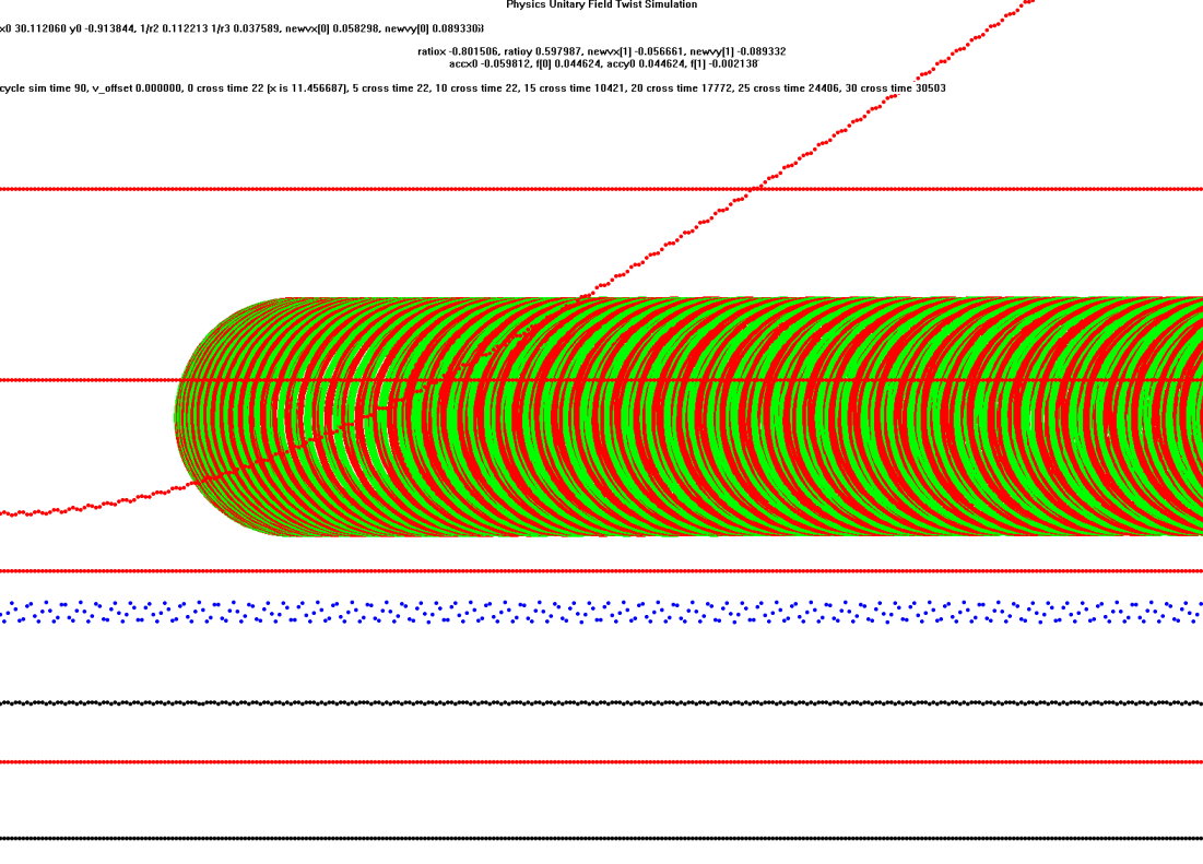
Well, it looked promising–qualitatively, it all added up, and everything behaved as expected.  But it’s a “close, but no cigar”.   The acceleration at each point should be proportional to 1/r^2, but after a large number of runs, it’s pretty clearly some other proportionality factor.  I’ve got some more checking to do, but looks like I don’t have the right animal here.  One thing is clear though–this model, which attracts and repels, is the first one that shows qualitatively correct behavior.  If twist rings have mass due to the twist distortion, this is the first model that shows it, even if the mass can’t be right.

So, I stepped back and ran through the list of assumptions, and see some flaws that might guide me to a better solution.  Many theories die in the real world because of the glossy effect, as in, I glossed over that and will deal with it later, it’s not a major problem.  I unintentially glossed over some problems with the model, and in retrospect I should have addressed them from the get-go.

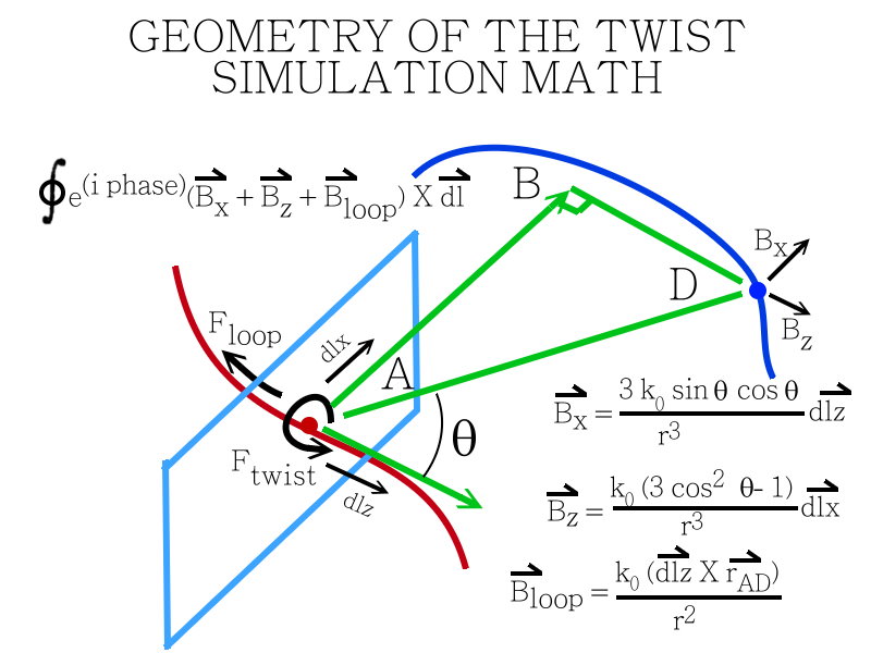
First, twist rings (as modelled in my simulation) have a real planar component, but twist through an imaginary axis.  The twist acts as an E field in the real space and as a magnetic field in the imaginary space.  The current hypothesis is that the loop experiences different field magnitudes from the source particle, and this causes a curvature change that varies around the loop.  The part of the loop that is further away will experience less curvature, the closer part more curvature (curvature is a function of the strength of the magnetic field from the source particle).  This simulation shows that if that is the model, you do indeed get an acceleration of the ring proportionate to the distance from the source particle–and the acceleration is toward the source particle–attraction!  If you switch the field to the negative, you get the same acceleration away–repulsion.  So far, so good, and the sim results made me think–I’m on the right track!  I still think I might be on the right track, but the destination is further away than I thought.

First, as I mentioned, the sim results seem to show pretty clearly that the acceleration is not the right proportionality (1/r^2).  That might just be a computational problem or just indicate the model needs some adjustments.  But there are some things being glossed over here.  First, while the model works regardless of how many particles act as a source, there is always one orientation where every point on the ring is equadistant from the source particle–in this case, there is no variation in curvature.  The particle would have to act differently depending on orientation.  It could be argued that the particle ring will always have its moment line up with the source field, and so this orientation will never happen–fine, but what happens when you have two source particles at different locations?  The line-up becomes impossible.  OK, let’s suppose some sort of quantum dual-state for the ring–and I say, I suppose that is possible, some kind of sum of all twist rings, or maybe a coherence emerges depending on where the source particles are, but then we no longer have a twist ring.  In addition, the theory fixes and patches are building up on patches, and I’d rather try some simpler solutions before coming back to this one.  The orientation problem is a familiar one–it shoots down a lot of geometrical solutions, including the old charge-loop idea.

Here’s another issue:  I make the assumption that there is a “near side” and a “far side”, which has the orientation problem I just mentioned–a corollary to that is that it also could get us in trouble as soon as relativity comes in play since near and far are not absolute properties in a relativistic situation).  I then get an attraction by assuming the field is weaker on the far side and thus there is less curvature.  The sim shows clearly the repulsion acceleration away from the source when this is done.  Then I cavalierly negated the field and Lo! I got attraction, just like I expected.  But I thought about this, and realized this doesn’t make physical sense–a case of applying a mathematical variation without thinking.  This would mean that the field caused *greater* curvature when the twist point is further away (the far side).  Uhh, that does not compute…

While not completely conclusive, this analysis points out first, that a solution cannot depend on source field magnitude variation alone within the path of the ring.  The equidistant ring orientation requires (more correctly, “just about” requires, notwithstanding some of the alternatives I just mentioned) that the solution work even if all neighborhood points on the ring have exactly the same source field magnitude.  In addition, there’s another more subtle implication.  The direction a particle is going to move has to come from a field vector–this motion cannot result from a potential function (a scalar)  because within the neighborhood of the ring, the correct acceleration must occur even if the potential function appears constant over the range of the twist ring.

This is actually a pretty severe constraint.  In order for a twist ring to move according to multiple source particles, a vector sum has to be available in the neighborhood of the twist ring and has to be constant in that neighborhood.  The twist ring must move either toward or away from this vector sum direction, and the acceleration must be proportionate to the magnitude of the vector sum.  Our only saving grace is the fact that this vector sum is not necessarily required to lie in R3, possible I3–but a common scalar imaginary field of the current version of the twist theory is unlikely to hold up.

Is the twist field theory in danger of going extinct even in my mind?  Well, yes, there’s always that possibility.  For one thing, I am assuming there will be a geometrical solution, and ignoring some evidence that the twist ring and other particles have to have a more ghostly (coherent linear sum of probabilities type of solution we see in quantum mechanics).  For another, my old arguments about field discontinuities pop up whenever you have a twist field, there’s still an unresolved issue there.

But, the driving force behind the twist field theory is E=hv.  A full twist in a background state is the only geometrical way to get this quantization in R3 without adding more dimensions–dimensions that we have zero evidence for.   Partial twists, reverting back to the background state, are a nice mechanism for virtual particle summations.  We do get the Lorentz transform equations for any closed loop solution such as the twist theory  if the time to traverse the loop is a clock for the particle.  And–the sim did show qualitative behavior.  Fine tuning may still get me where I want to go.

Agemoz

Twist Ring Acceleration Sim Results

July 7, 2013

The initial measurements are in, and still look promising.  To recap, one stable form of the twist in the Unitary Twist Field theory is in a ring where the twist curves on itself as a combination of the electrostatic 1/r^2 and magnetic field 1/r^3 strengths (this ratio is defined by the fine structure constant).  There are potentially many solutions, but only one possible planar solution other than the linear twist–the twist ring.  I posited that if this were true, placing a twist ring in an external electrostatic field would cause the curvature to vary depending on the distance from a source charged particle.  Computing this analytically is a challenge, yielding a 24 term LaGrange differential equation of motion, so I decided to do this iteratively.

This was a lot easier, and has yielded promising results that suggest I might be on the right track.  The initial sims showed correct qualitative behavior with repulsion or attraction depending on the external field polarity, and I could visually see the correct acceleration behavior.

Next, I added quite a bit of numerical analysis code to the sim of the twist ring path, and was able to verify that a linearly varying field will cause the path of motion to accelerate at a constant rate–and that this acceleration is proportionate to the strength of the field within some level of accuracy.  Much more needs to be done to confirm these measurements, but the initial results show that this type of model (twist ring) will give electrostatic behavior.  Here’s a pic where you can see the displacement with time (the parabolic curve).  Following that, you’ll see my initial data set along with the Mathematica solution for the first three crossing points of the parabola–more computations will be done to establish that this really is a parabola.

From here, I will see if the correct mass results from the ratio of the strength of the 1/r^2 component to the 1/r^3 component in an electron.  There should also be other twist loop solutions possible in 3D, I’ve limited myself to the easiest (planar) solution to start.

Agemoz

twist_ring_measured_repel

Here’s the initial sim time crossing points, along with the Mathematica solve solutions:

Running the Unitary Field Twist simulation to numerically derive the change in x as
a field is asserted on a 1/r^2 - 1/r^3 twist ring.  The field affects the curvature
(magnetic component).  The result generates the qualitative expected movement as if
there was a central force effect (q^2/r^2).  These results are an attempt to measure
the acceleration factor as a function of relative field strength (magnetic to
electrostatic).

Since the equations of motion due to the 1/r^2 - 1/r^3 equation in a linear field
were 24 parameter LaGrange equations of motion, I attempted to get an analytic
solution by examining the iterative numerical results.

Here is the result for 1:1 (1/r^2 to 1/r^3) field strength at distance 10 with
radius 1.5 and ring velocity 0.10545 and source field strength factor .0005.
The sim showed a cycle time of about 90.

field strength 0.00025
22:  11.457            (doesnt start at zero because cycle max x is not at zero)
14545: 15
25213: 20
34448: 25
43234: 30

using the first 3 terms in quadratic solution, I get
x = 8.92 10^9 * t^2 + .000114 * t + 11.455

field strength 0.0005
22:  11.457            (doesnt start at zero because cycle max x is not at zero)
10421: 15
17772: 20
24406: 25
30503: 30

using the first 3 terms in quadratic solution, I get
x = 1.912 10^8 * t^2 + .000141 * t + 11.454

field strength 0.0010
22:  11.457            (doesnt start at zero because cycle max x is not at zero)
7372: 15
12572: 20
17233: 25
21626: 30

using the first 3 terms in quadratic solution, I get
x = 3.82 10^8 * t^2 + .000200 * t + 11.453

More terms need to be computed, but there is a clear linear proportionality to the 
acceleration component of the curve, consistent with the expected electrostatic
relation of field strength proportionate to the acceleration of the destination
particle.